Introduction

In audio processing, Equalization (EQ) is the process of adjusting the relative balance of frequency components in an audio signal. A Parametric EQ is a type of audio equalizer that allows full control over three components of each filter band in the EQ; frequency, gain, and bandwidth. This can be contrasted against other equalizers like graphical equalizers (which you might find in your car stereo for example) that only provides gain control for bands at a fixed frequency interval and have a fixed bandwidth for each band. This makes Parametric EQs a very versatile audio processing tool in the studio, from broad stroke frequency adjustments like boosting the bass and treble of the master bus for a more exciting mix, or surgically cutting harsh resonant frequencies often found in drum cymbals.

I created a digital Parametric EQ audio plugin for digital audio workstations (DAWs) targetting Steinberg’s Virtual Studio Technology (VST3) plugin format. This project utilizes Oli Larkin’s edition of the Cockos' IPlug audio plugin framework and Cairo 2D graphics library. This EQ implements Robert Bristow-Johnson’s (RBJ) biquad filters, providing a selection of low cut, high cut, low shelf, high shelf, and peaking EQ filters, and also allows for an unlimited number of filter bands.

Demo

Operation

In this plugin, the user has the ability to implement any number of digital filters they want to form the overall EQ. Each band has three main controls:

• The frequency of the band, which may mean the center frequency or the corner frequency (-3 dB) depending on the filter type

• The gain of the band, which when applicable (depending on filter type) will control how much that band is adding or subtracting for its bandwidth.

• The ‘Q’ of the band is a sort of coarse control for bandwidth. This can control how wide or narrow the frequency bandwidth is for the peaking filter, or emphasize resonant bumps seen in the high/low pass and shelving filters.

Bands can be added via ctrl + left clicking, their controls can be accessed by clicking the colored circle that’s a part of their band, and can be deleted by pressing the red ‘x’ in the corner of their controls. The mouse can be used to drag the band around (controlling the ‘freq’ by moving along the x-axis, and controlling the ‘gain’ by moving along the y-axis). The mouse wheel controls the ‘Q’ of the band. All of these parameters can also be accessed by the knobs at the bottom of the screen. Additionally, double clicking on a band will disable it (which can be seen by it becoming grayed out), and won’t contribute to the processing of the EQ.

Audio Processing

The RBJ Biquads are a general 2nd order infinite impulse response (IIR) digital filter. They are implemented in code with the following Direct-Form 1 difference equation:

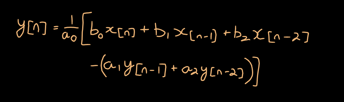
IIR filters are characterized by their feedback path (as seen by the y[n-1] and y[n-2] terms) where their impulse response never decays to zero. Their computational complexity is (in general) significantly lower than their FIR counterparts, requiring fewer computations per time step and less memory.

The various filter coefficients can be computed depending on the desired type of filter one wants to implement. More detail on how these coefficients are computed can be found in RBJs original post here, where he outlines designs for the high/low pass, high/low shelf, and peaking filter designs utilized in this project.

Additionally, this plugin computes the amplitude response of the EQ, allowing the user to interact with a visual representation of the filters that they have configured.

Equalizer Amplitude Response

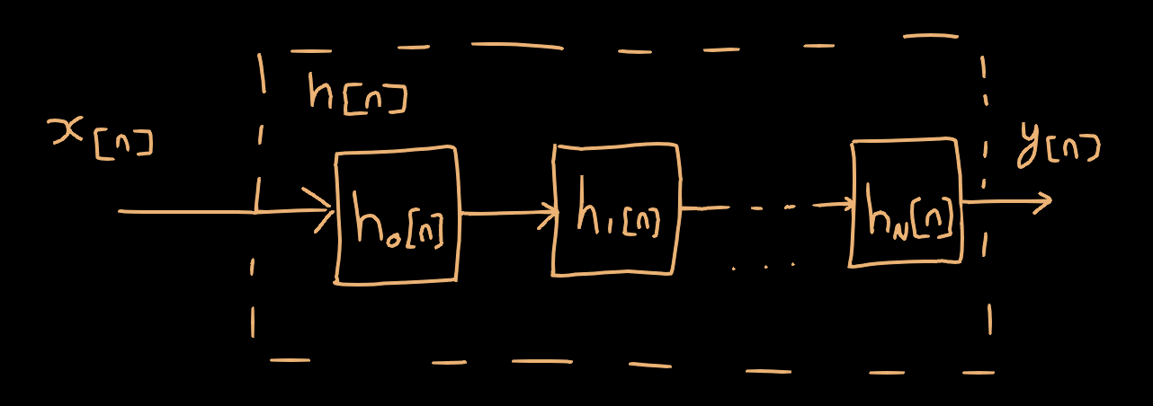
The graphical gain vs. frequency plot that the user sees and interacts with is produced by computing the amplitude response (or magnitude frequency response) portion of a Bode Plot for the cascaded filter bands configured by the user. The amplitude response provides the frequency-gain that the filter applies to an arbitrary input signal as a function of frequency. See below for a diagram of the cascaded filter stages of the equalizer, where x[n] is our time-domain input signal, y[n] is the time-domain output signal, and h[n] is the overall time-domain transfer function of the system, made up of serially cascaded filter bands each with their own transfer functions.

Here I will go into some details about how we can compute and display the amplitude response for this system.

Frequency Response

First, we will look at computing the frequency response for an arbitrary system, and how the amplitude response relates to it. Then we can apply it to our biquad filters.

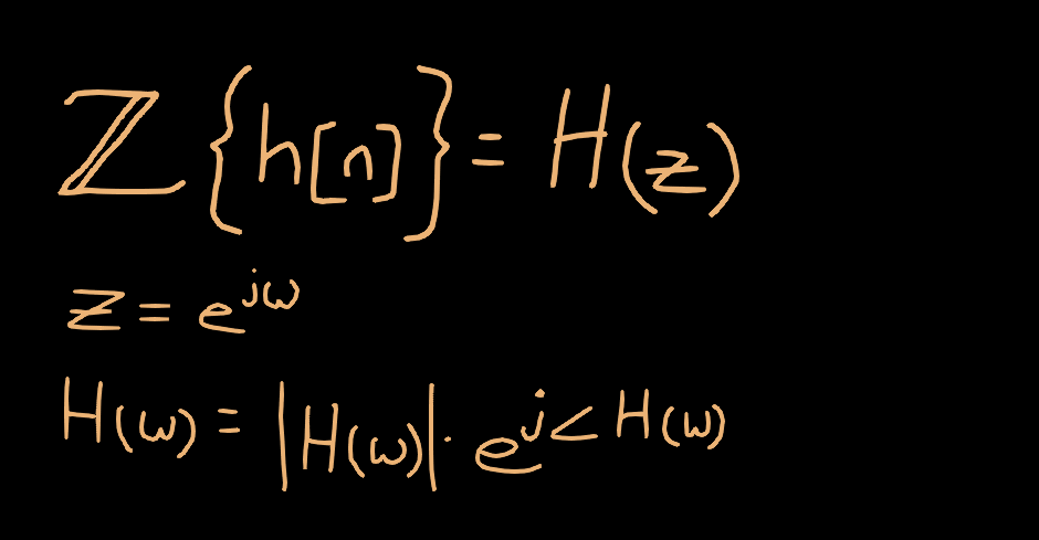
A discrete time-domain transfer function h[n] is related to its frequency domain representation H(z) through the z-transform. A discrete linear time-invariant (LTI) system characterized by the transfer function H(z) has a frequency response given by the following (in polar form):

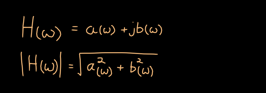
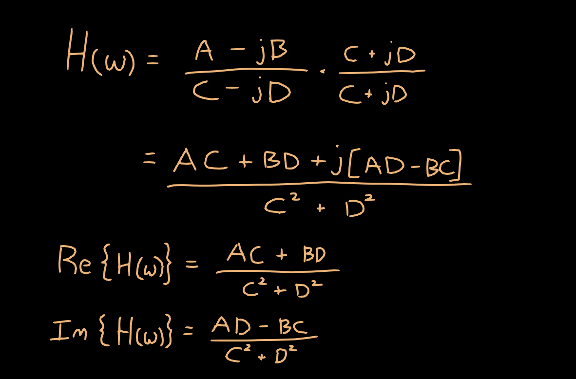
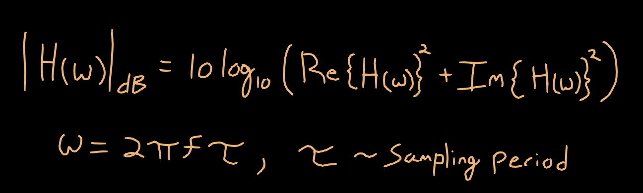
The amplitude response is given by |H(ω)|. Given the complex-valued transfer function, this can be computed as follows:

Next, we need to compute the overall amplitude response of our system. Our system is made up of multiple filters cascaded together. Since each one is an LTI system, it is very easy to combine them into a manageable result when working in the frequency domain. Multiple cascaded LTI systems are characterized by the convolution of their discrete-time transfer functions, and consequently the multiplication of their frequency domain transfer functions:

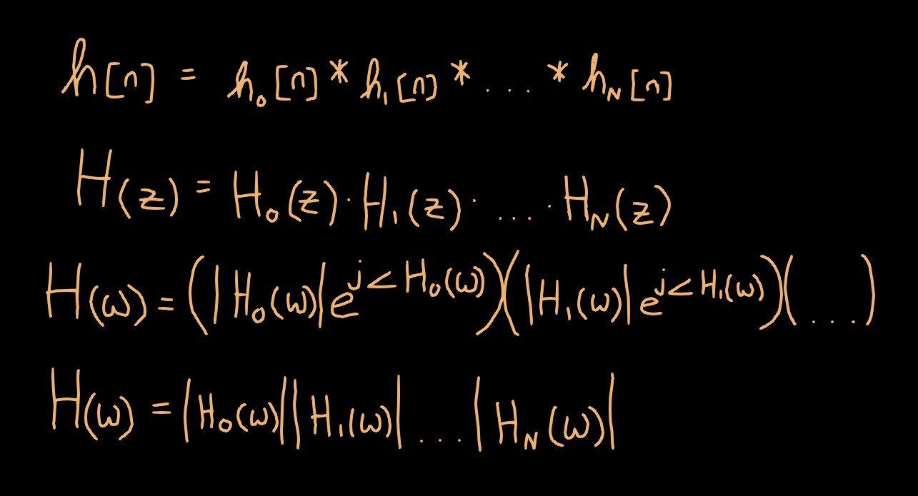
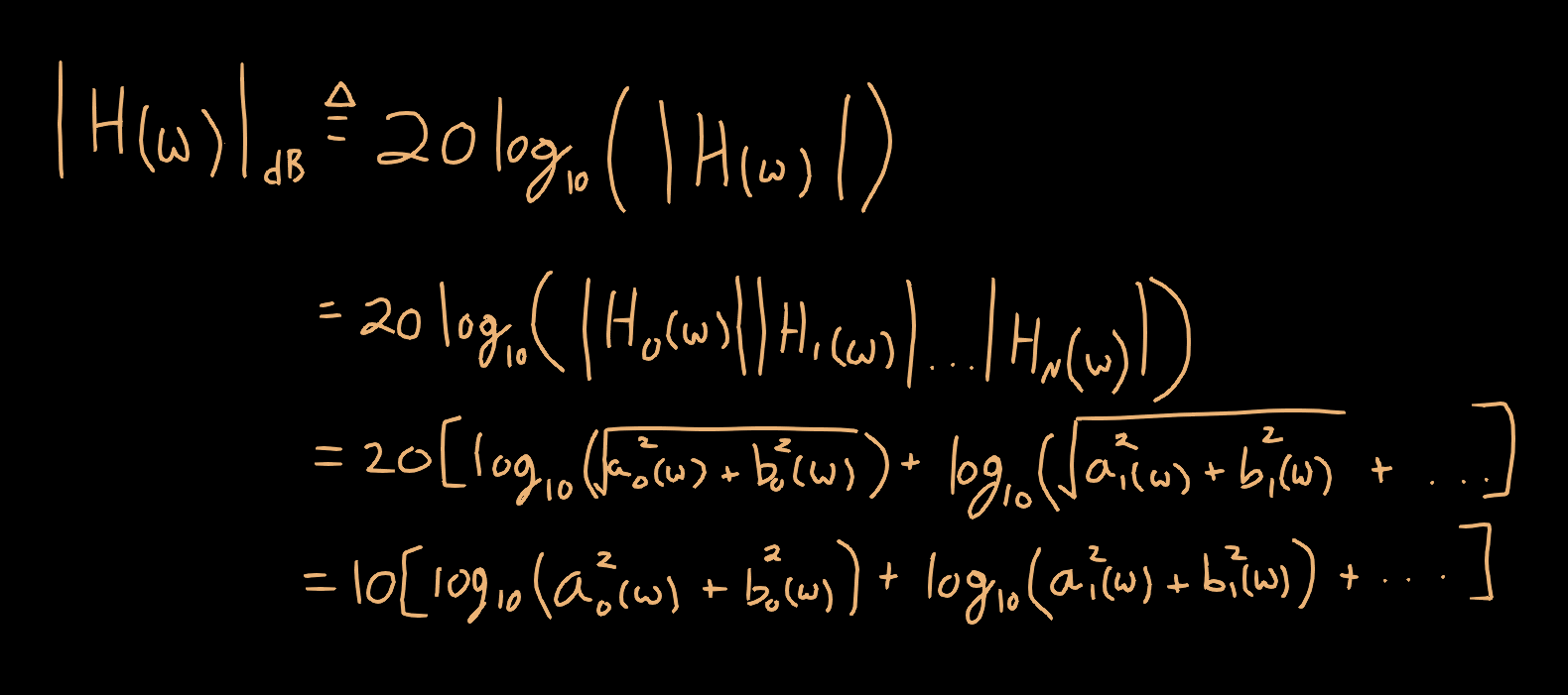
Thus, to compute the amplitude response of the cascaded system, we can compute the amplitude response of the individual transfer functions multiplied together. Finally, we need to convert the gain described as a scaling factor into a gain in decibels (dB). This also results in a nice little simplification that makes computing the overall amplitude response a bit easier, by only needing to add the gains (in dB) instead of multiplying the complex-valued results together.

Response of Biquad Filters

The discrete transfer function for each RBJ biquad filter band is provided as follows

Now, we can determine the frequency response of the biquad. We will use Euler’s formula to expand the complex exponentials into their sinusoidal components, and a couple trig identities for simplification.

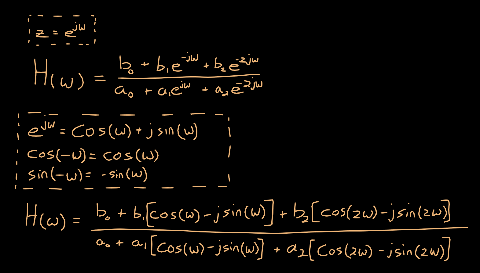
Next, we can combine our real and imaginary components to get the numerator and denominator into standard form.

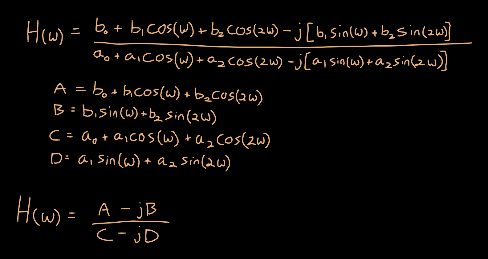
Now, we are in a little bit of a pickle. We need to get this entire expression into standard form so we can use it to compute the amplitude response, but the division of two complex numbers makes this a bit tricky. We can multiply and divide by the complex conjugate of the denominator to get the denominator into a purely real quantity.

This is great! Now that we have this in standard form, we can use our previous formulas for computing the gain. Then, we need to make a substitution for ω to convert from angular frequency to discrete ordinary frequency f.

Plotting the Amplitude Response

For this EQ, we want to plot both the amplitude response of each individual filter, as well as the response of the whole system. We can do this by testing the filters at varying frequency bins (representing our x-axis) to compute the gain for each filter at each bin, then combine them to compute the overall response of the EQ. Then we can plot the gains as a function of frequency to create a visualization of each filter band as well as the complete response. We want to display our x-axis as a logarithmic scale, so we need to convert our x-coordinates to a frequency on a logarithmic scale instead of a linear scale. For the sake of simplicity, in the pseudo code example below we will create a frequency bin for each pixel on the x-axis, and we will also avoid interpolating from bin to bin.

 1
 2
 3
 4
 5
 6
 7
 8
 9
10
11
12
13
14
15
16
17
18
19
20
21
22
23
24
25

float minFreqHz = 20.0f;
float maxFreqHz = 20000.0f;
for(int xPos = 0; xPos < width; ++xPos) {
    
    float freq = convert_xpos_to_freq_log10(xPos, windowWidth, minFreqHz, maxFreqHz);
    float totalMagDB = 0.0f;
    for(size_t biquadIdx = 0; biquadIdx < biquads->len; ++biquadIdx) {
        Biquad *biquad = biquads + biquadIdx;

        float magDB = biquad_calc_magdb_at_freq(biquad, freq, samplingPeriod);
        int yPos = convert_magdb_to_ypos(magDB);

        if(biquad->isActive) {
            draw_px(xPos, yPos, biquad->color);
            totalMagDB += magDB;
        } else {
	    // NOTE(Brett): Doesn't contribute to total amplitude response
            draw_px(xPos, yPos, COLOR_GREY);
        }
    }

    draw_px(xPos, yPos, totalResponseColor);
}

Where biquad_calc_magdb_at_freq computes the gain at the frequency being queried.

Future Plans

In the future, I would like to add a phase plot for fun. This isn’t something I’ve seen on digital EQs before, and it could be very handy. If you aren’t listening carefully or don’t understand the phenomena, filters (depending on the design) can introduce frequency-dependent phase shifts, which can create phase cancellation between multiple sources that is very difficult to diagnose. This will be most commonly encountered when trying to do processing on different sources with lots of low frequency information (e.g., kick drum and bass guitar) which causes phase cancellation, reducing their impact.

I would also like to try incorporating a live spectrum analyzer, so you can see the frequency content of an input source and visualize the effect EQ changes are having on the output. This would also give me an excuse to try my hand at writing an FFT butterfly from scratch.